Overfitting in Backtests: How to Spot It Before It Costs You

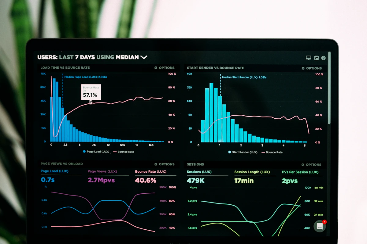
Every trader who's spent a weekend curve-fitting a strategy in a backtesting platform has felt it: the moment the equity curve turns into a smooth 45-degree line and you think you've found the holy grail. Then you go live, or you run it on data the optimizer never saw, and it falls apart. That's overfitting in backtesting — and it's probably the single biggest reason retail and even funded traders lose money on "proven" systems. This isn't a niche academic concern. It's the mechanical, almost guaranteed outcome of running enough parameter combinations against a finite chunk of history.

Here's what actually happens: you don't set out to overfit. Nobody opens a strategy builder thinking "I'm going to fool myself today." You just want a slightly better entry filter, so you test five moving average lengths. Then three RSI thresholds. Then two stop-loss multiples. Before you know it, you've tested 200+ combinations on the same 18 months of ES futures data, and the "best" one isn't skill — it's noise that happened to line up with that specific stretch of price history.

What Overfitting In Backtesting Actually Looks Like

Overfitting is when a strategy's rules are tuned so closely to a specific historical dataset that they capture random noise instead of a real, repeatable market behavior. The backtest looks fantastic. The forward performance doesn't, because the noise pattern that made your parameters "optimal" doesn't repeat — it was never a pattern to begin with, just a coincidence in that sample. The tell is usually a strategy with too many moving parts relative to how much data you tested it on. David H. Bailey, Marcos López de Prado, and their co-authors formalized this in their research on backtest overfitting: they built a simulator that exhaustively explores parameter combinations on pure random walk data — data with zero real structure — and it still reliably produces "optimal" strategies that look profitable in-sample and even hold up reasonably well out-of-sample, purely by chance, given enough trials. Their point is blunt: if you try enough variations, you will find something that looks good, whether or not there's anything real underneath it. That paper is worth reading directly if you want the math — Statistical Overfitting and Backtest Performance lays it out with an online simulator to demonstrate it.

Parameter Count vs. Sample Size: The Core Math Problem

This is the part beginners get wrong most often: they treat "more filters" as automatically "more robust." It's backwards. Every additional parameter you add — another moving average, another volatility filter, another time-of-day restriction — is another degree of freedom the optimizer can use to fit your specific historical sample rather than the underlying market behavior. Think about it in plain terms. If you have 300 trading days of data and you're optimizing four parameters, each with even a modest range of values, you might be testing thousands of combinations against a dataset that only contains a few hundred independent observations (and futures returns are autocorrelated day to day, so your effective sample size is even smaller than the raw day count suggests). You're not finding an edge. You're finding the combination that happened to fit the noise in that particular window best. A rough rule some quant researchers use: you want a meaningful multiple of data points per free parameter — not two or three, but dozens, ideally hundreds — before you can trust that an optimized value reflects something durable. A strategy with 8-10 tunable inputs (moving average length, ATR multiplier, RSI period, RSI threshold, session filter, day-of-week filter, stop distance, target distance, and so on) run against a single year of 5-minute ES data is almost certainly overfit no matter how good the equity curve looks.

In-Sample vs. Out-of-Sample: Doing the Split Properly

The standard defense against overfitting is splitting your data into an in-sample (IS) period, where you develop and optimize the strategy, and an out-of-sample (OOS) period, which the strategy never touches during development. If performance holds up reasonably well on the OOS segment, that's a real (though not conclusive) signal. Where people mess this up:

• Peeking. You "just glance" at OOS results, tweak a parameter, retest. Now your OOS data has silently become IS data. This is the single most common way traders fool themselves.
• Single split, no repetition. One IS/OOS split tells you how the strategy did on one particular slice of history. It doesn't tell you the split wasn't a lucky one. Walk-forward testing — repeatedly rolling the IS/OOS boundary forward through time and re-optimizing — gives a far more honest picture of how a strategy performs across different regimes.
• OOS period too short or too easy. An OOS window that's 10% of your data, or that happens to be a smooth trending month, doesn't stress-test anything. You want an OOS period that covers different volatility regimes: a chop period, a strong trend, a high-volatility event window (think a CPI print or an FOMC day for futures traders).
• Data snooping across strategies. This is subtler — if you've tested 50 strategy ideas over the years on the same futures dataset and only kept the ones that worked, you've overfit at the "which idea did I keep" level even if each individual strategy was tested cleanly. This is exactly the multiple-trials problem the deflated Sharpe ratio was built to address.

The Deflated Sharpe Ratio: Correcting for How Many Times You Tried

A standard Sharpe ratio doesn't know how many strategy variants you tested before landing on the one you're looking at. If you test 500 random parameter combinations, the best one will have an inflated Sharpe ratio purely from the selection process — even if none of the 500 had any real edge. This is the same statistical problem as p-hacking in scientific research: run enough trials, and something will clear your significance bar by chance. The deflated Sharpe ratio (DSR), developed by Bailey and López de Prado, adjusts the observed Sharpe ratio downward based on three things: the number of independent trials you ran to find this strategy, the variance across those trials' Sharpe ratios, and the non-normality (skewness and kurtosis) of the strategy's return distribution — since fat-tailed, negatively skewed returns (very common in trend and breakout systems) make a standard Sharpe ratio overstate the strategy's statistical significance. Practically, the DSR asks: "given how many shots you took, what's the probability this Sharpe ratio is genuinely above zero skill, and not just the best of many random draws?" A follow-up implementation and explainer worth reading is The Deflated Sharpe Ratio in Practice, which walks through the formula and a working Python implementation. You don't need to compute DSR by hand to get the lesson: the more variants you tried, the more skeptical you should be of the winner. A strategy that's the best of 3 clean, economically-motivated ideas deserves far more trust than the best of 3,000 auto-optimized parameter combinations, even if the raw backtest Sharpe ratios look identical.

Practical Signs Your Backtest Is Overfit

A few patterns show up over and over in overfit systems:

1. The equity curve is suspiciously smooth, with almost no flat or drawdown periods across years of data. Real markets don't behave that consistently.
2. Small changes to a parameter (say, moving an ATR multiplier from 2.0 to 2.2) cause large swings in backtested profitability. A robust strategy should perform similarly across a reasonable neighborhood of parameter values — this is sometimes called a "parameter plateau" versus a "parameter spike."
3. The strategy relies on a handful of huge winning trades that, if removed, turn the whole backtest negative. That's concentration risk disguised as an edge.
4. Performance is dramatically better on one specific futures contract, session, or year than on anything else, with no clear structural reason why.
5. You needed many conditional filters (day-of-week, time-of-day, volatility regime, etc. stacked together) to get the equity curve looking clean.

Why This Matters More for Prop Firm Accounts

If you're trading a funded account — Apex Trader Funding, Topstep, or any of the other prop firms — overfitting isn't just an abstract statistics problem, it's the thing that gets your account breached. Prop firm evaluations give you a fixed, short window (Apex's evaluation accounts, for example, run on a 30-calendar-day clock with defined trailing drawdown limits) and a trailing maximum loss limit that only moves in your favor as your balance grows. A strategy that looked great in a backtest because it was tuned to a specific historical stretch has no reason to keep working during your live evaluation window, and a string of losses from a strategy that's secretly noise-fitted is exactly how funded accounts get blown. You can check the current rule structure directly on Apex's site, but the core lesson applies to any firm: your live trading window is, by definition, out-of-sample data relative to whatever period you backtested on. If your strategy wasn't validated out-of-sample before you went live, your funded evaluation is doing that validation for you — with real consequences attached.

Building a Backtest Process That Resists Overfitting

None of this means backtesting is useless or that optimization is forbidden. It means you need discipline around the process:

• Keep parameter counts low. Fewer, economically justified inputs beat many curve-fit ones.
• Reserve a true out-of-sample window and don't touch it until the strategy design is frozen.
• Use walk-forward analysis instead of a single static split whenever you have enough data.
• Test across multiple instruments or contract months where the underlying logic should apply, not just the one dataset you developed on.
• Track how many variants you tested, even informally, so you have an honest sense of how "found" versus "designed" your final strategy really is.
• Favor strategies with a parameter plateau — where nearby parameter values still perform reasonably — over ones with a sharp performance spike at one specific setting.

Frequently Asked Questions

What's the difference between curve-fitting and legitimate optimization?

Legitimate optimization adjusts a small number of economically justified parameters within a reasonable range and checks for stability across nearby values and multiple time periods. Curve-fitting is when you search a large parameter space until you find the single combination that maximizes historical profit, without regard to whether that combination makes logical sense or holds up in neighboring parameter values.

How much out-of-sample data do I actually need?

There's no single magic number, but as a floor, most practitioners want an OOS period that's a meaningful fraction of the in-sample period (commonly 20-30%) and that spans at least one full market cycle — meaning both trending and choppy conditions, and ideally a high-volatility stretch. A one-month OOS test after a two-year in-sample optimization tells you very little.

Can a strategy with a low backtested Sharpe ratio still be good?

Yes, and this trips people up. A modest, stable Sharpe ratio achieved with few parameters and consistent out-of-sample performance is more trustworthy than a spectacular Sharpe ratio produced by heavy optimization over many trials. The deflated Sharpe ratio framework exists precisely because raw Sharpe ratios don't account for how many attempts it took to find the "best" version.

The uncomfortable truth is that a backtest can never prove a strategy works — it can only fail to prove that it doesn't. Overfitting is what happens when you mistake the absence of failure in one historical sample for genuine skill. Treat every backtest with that skepticism, keep your parameter count honest relative to your data, and let out-of-sample results — real ones, not ones you peeked at — do the talking.